Convolution kernels and PSFs

The point spread function (PSF) describes the two-dimensional distribution of light in the telescope focal plane for the astronomical point sources. To get reliable multiwavelength photometric SED from a set of multiband images, especially in the analysis of spatially resolved SEDs of galaxies, it is important to homogenize the spatial resolution (i.e., PSF size) of those images before extracting SEDs from them. This process of homogenizing the PSF size of multiband images is called PSF matching. The final/target spatial resolution to be achieved is the one that is the lowest (i.e., worst) among the multiband images being analyzed. Commonly, PSF matching process of multiband images is done by convolving the images that have higher spatil resolution (i.e., smaller PSF size than the target PSF) with a set of pre-calculated convolution kerenels. The convolution kernel for matching a pair of two PSFs is derived from the ratio of Fourier transforms (e.g., Gordon et al. 2008; Aniano et al. 2011).

For PSF matching process, piXedfit_images module uses convolution kernels from Aniano et al. 2011 that are publicly available at this website. The available kernels cover various ground-based and spaced-based telescopes, including GALEX, Spitzer, WISE, and Herschel. Besides that, Aniano et al. 2011 also provide convolution kernels for some analytical PSFs that includes Gaussian, sum of Gaussians, and Moffat. Those analytical PSFs are expected to be representative of the net (i.e., effective) PSFs of ground-based telescopes.

To associate the PSFs of SDSS and 2MASS (which are not explicitely covered in Aniano et al. 2011) with the analytical PSFs of Aniano et al. 2011, we have constructed empirical PSFs of the 5 SDSS bands and 3 2MASS bands and compare the constructed empirical PSFs with the analytical PSFs from Aniano et al. 2011. We find that the empirical PSFs of SDSS \(u\), \(g\), and \(r\) bands are best represented by double Gaussian with FWHM of 1.5’’, while the other bands (\(i\) and \(z\)) are best represented by double Gaussian with FWHM of 1.0’’. For 2MASS, all the 3 bands (\(J\), \(H\), and \(\text{K}_{\text{S}}\)) are best represented by Gaussian with FWHM of 3.5’’. Construction of these empirical PSFs is presented in Appendix A of Abdurro’uf et al. (2020, submitted). The empirical PSFs are available at this Github page. For consistency, the piXedfit_images use those analytical PSFs to represent the PSFs of SDSS and 2MASS and use the convolution kernels associated with them whenever needed.

By default, when external kernels are not provided by the user, piXedfit_images module will use the kernels from Aniano et al. 2011. For flexibility, the users can also input their own kernels to piXedfit_images.

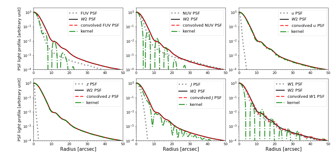
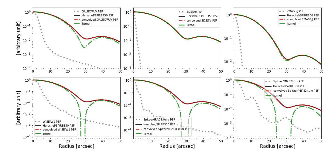
Figures below show a demonstration of the performance of some convolution kernels used in the piXedfit_images module. In the top figure, the performance of the convolution kernels used to achieve the spatial resolution of WISE/\(W2\) is demonstrated. Different panels show different initial PSFs. In the first row from the left to right, we show the convolution results from initial PSFs of GALEX/FUV, GALEX/NUV, and SDSS/\(u\), respectively. The second row, from left to right, we show the result for SDSS/\(z\), 2MASS/\(J\), and 2MASS/\(W1\), respectively. In the bottom figure, the performance of the convolution kernels used to achieve the spatial resolution of Herschel/SPIRE350 is demonstrated. In the first row from the left to right, we show the convolution results from initial PSFs of GALEX/FUV, SDSS/\(u\), and 2MASS/\(J\), respectively. The second row, from left to right, we show the result for WISE/\(W1\), Spitzer/IRAC \(8.0\mu \text{m}\), and Spitzer/MIPS \(24\mu \text{m}\), respectively. The figures shows that the performance of the convolution kernels is very good, evidenced from the good matching between the shapes of the convolved PSFs and the target PSF.

For the characteristic PSFs of the imaging data that can be analyzed with the current version of piXedfit, please see the description in this page.