Get maps of spatially resolved properties

Once we finished SED fitting to all spatial bins in the galaxy, we can construct maps of properties from the collection of those fitting results (in FITS files). For this, we can use piXedfit.piXedfit_fitting.maps_parameters() function in the piXedfit_fitting module. Please see the API reference here for more information about this function. An example of script to get the maps properties is shown below.

from piXedfit.piXedfit_fitting import maps_parameters

fits_binmap = "pixbin_corr_specphoto_fluxmap_ngc309.fits"
hdu = fits.open(fits_binmap)
nbins = int(hdu[0].header['NBINSPH'])
hdu.close()

bin_ids = []
name_sampler_fits = []
for ii in range(0,nbins):
        bin_ids.append(ii)
        name = "mcmc_bin%d.fits" % (ii+1)
        name_sampler_fits.append(name)

fits_fluxmap = "corr_specphoto_fluxmap_ngc309.fits"
name_out_fits = "maps_properties.fits"
maps_parameters(fits_binmap=fits_binmap, bin_ids=bin_ids, name_sampler_fits=name_sampler_fits,
                fits_fluxmap=fits_fluxmap,refband_SFR=0, refband_SM=11, name_out_fits=name_out_fits)

We can then make plots from the maps stored in the output FITS file.

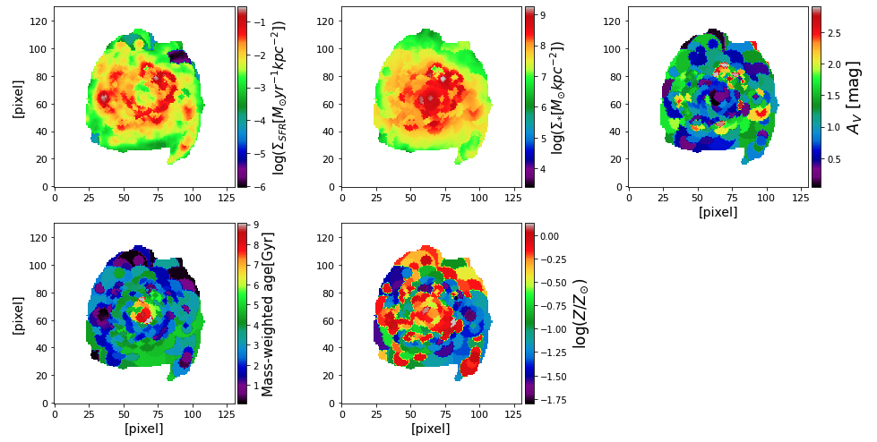
maps = fits.open("maps_properties.fits")
gal_region = maps['galaxy_region'].data

# calculate physical size of a single pixel
from piXedfit.piXedfit_images import kpc_per_pixel

z = float(maps[0].header['gal_z'])
arcsec_per_pixel = 1.5                           # pixel size in arcsec
kpc_per_pix = kpc_per_pixel(z,arcsec_per_pixel)

rows, cols = np.where(gal_region == 0) # get pixels outside the galaxy's region of interest

# stellar mass surface density
map_prop_SM = np.log10(np.power(10.0,maps['pix-log_mass-p50'].data)/kpc_per_pix/kpc_per_pix)
map_prop_SM[rows,cols] = float('nan')

# surface density of SFR
map_SFR = np.log10(np.power(10.0,maps['pix-log_sfr-p50'].data)/kpc_per_pix/kpc_per_pix)
map_SFR[rows,cols] = float('nan')

# Av dust attenuation
map_Av = 1.086*maps['bin-dust2-p50'].data
map_Av[rows,cols] = float('nan')

# stellar metallicity
map_logzsol  = maps['bin-logzsol-p50'].data
map_logzsol[rows,cols] = float('nan')

# Mass-weighted age
map_mw_age  = np.power(10.0,maps['bin-log_mw_age-p50'].data)
map_mw_age[rows,cols] = float('nan')

# plotting
from mpl_toolkits.axes_grid1 import make_axes_locatable

fig1 = plt.figure(figsize=(14,7))

###=> SFR surface density
f1 = fig1.add_subplot(2, 3, 1)
plt.ylabel('[pixel]', fontsize=14)
plt.setp(f1.get_xticklabels(), fontsize=11)
plt.setp(f1.get_yticklabels(), fontsize=11)

plt.imshow(map_SFR, origin='lower', cmap='nipy_spectral')
ax = plt.gca()
divider = make_axes_locatable(ax)
cax = divider.append_axes("right", size="5%", pad=0.05)
cb = plt.colorbar(cax=cax)
cb.set_label(r'log($\Sigma_{SFR}[M_{\odot}yr^{-1}kpc^{-2}]$)', fontsize=15)


###=> stellar mass surface density
f1 = fig1.add_subplot(2, 3, 2)
plt.setp(f1.get_xticklabels(), fontsize=11)
plt.setp(f1.get_yticklabels(), fontsize=11)

plt.imshow(map_prop_SM, origin='lower', cmap='nipy_spectral')
ax = plt.gca()
divider = make_axes_locatable(ax)
cax = divider.append_axes("right", size="5%", pad=0.05)
cb = plt.colorbar(cax=cax)
cb.set_label(r'log($\Sigma_{*}[M_{\odot}kpc^{-2}]$)', fontsize=15)

###=> AV dust attenuation
f1 = fig1.add_subplot(2, 3, 3)
plt.xlabel('[pixel]', fontsize=14)
plt.setp(f1.get_xticklabels(), fontsize=11)
plt.setp(f1.get_yticklabels(), fontsize=11)

plt.imshow(map_Av, origin='lower', cmap='nipy_spectral')
ax = plt.gca()
divider = make_axes_locatable(ax)
cax = divider.append_axes("right", size="5%", pad=0.05)
cb = plt.colorbar(cax=cax)
cb.set_label(r'$A_{V}$ [mag]', fontsize=18)

### mass-weighted age
f1 = fig1.add_subplot(2, 3, 4)
plt.xlabel('[pixel]', fontsize=14)
plt.ylabel('[pixel]', fontsize=14)
plt.setp(f1.get_xticklabels(), fontsize=11)
plt.setp(f1.get_yticklabels(), fontsize=11)

plt.imshow(map_mw_age, origin='lower', cmap='nipy_spectral')
ax = plt.gca()
divider = make_axes_locatable(ax)
cax = divider.append_axes("right", size="5%", pad=0.05)
cb = plt.colorbar(cax=cax)
cb.set_label('Mass-weighted age[Gyr]', fontsize=15)

### stellar metallicity
f1 = fig1.add_subplot(2, 3, 5)
plt.xlabel('[pixel]', fontsize=14)
plt.setp(f1.get_xticklabels(), fontsize=11)
plt.setp(f1.get_yticklabels(), fontsize=11)

plt.imshow(map_logzsol, origin='lower', cmap='nipy_spectral')
ax = plt.gca()
divider = make_axes_locatable(ax)
cax = divider.append_axes("right", size="5%", pad=0.05)
cb = plt.colorbar(cax=cax)
cb.set_label(r'log($Z/Z_{\odot}$)', fontsize=17)

plt.subplots_adjust(left=0.07, right=0.95, bottom=0.1, top=0.98, hspace=0.2, wspace=0.3)
plt.show()

We can then get a plot as shown below.